Retinal Fundus Image Enhancement With Image Decomposition

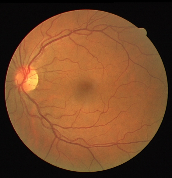
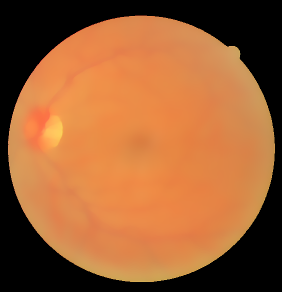
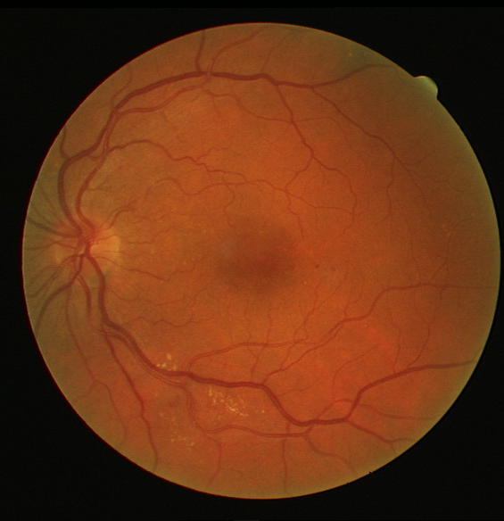
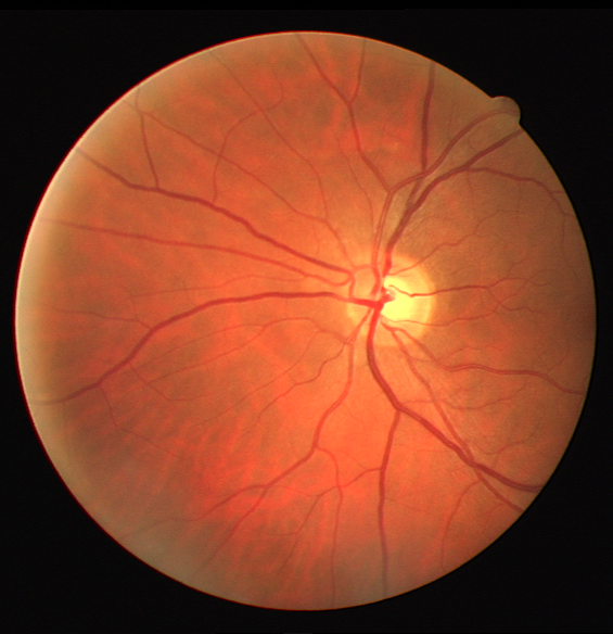
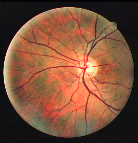
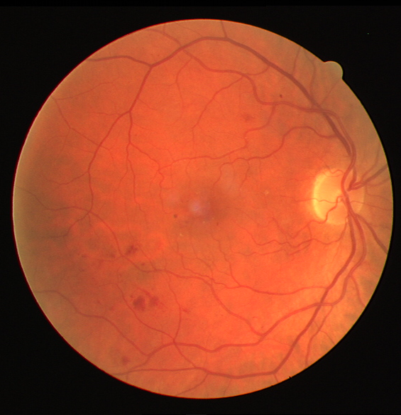
Retinal fundus photography is a non-invasive method to check for symptoms and other features related to diseases like diabetic retinopathy, age-related macular degeneration, cardiovascular disease. The main features to look out for are the vascular structure, lesions, optic disc, microaneurysms, etc. These depend on high quality fundus images to be processed properly. However, many such images are clinically unsatisfactory because of human error and electronic noise in the imaging instrument. The main problems are: non-uniform illumination, low contrast and noise.

Some common image enhancement methods are Histogram Equalization(HE) and Contrast Limited Adaptive Histogram Equalization(CLAHE). HE is performed over the entire image’s histogram and thus works over the entire contrast, rendering it in-effective for fundus image enhancements, where the contrast improvement requirements are regional. CLAHE performs better in this regard, because it can suppress noise in near-constant regions. Illumination correction happens simultaneously in this step. However, the individual color layers can still be enhanced more.

Proposed Method

In the CLAHE method, there is significant improvement in contrast, because of which vasculature of the fundus images becomes very clear. But there are still some dark spots and blobs, showing uneven illumination. The method used in this project uses a global noise estimation based image decomposition method to divide the input image into three layers, i.e., the base, detail, and noise layers. Then the base layer is corrected in HSV space, detail layer is enhanced and then they are combined back. Noise layer is rejected.

Image Decomposition

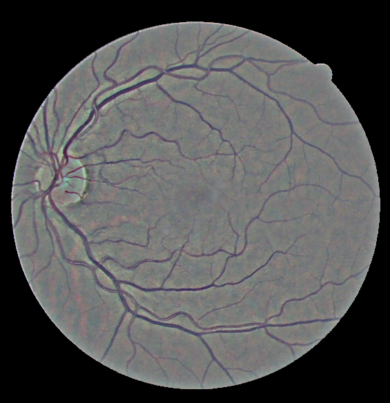
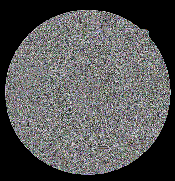
Total variation based structure decomposition method is used to separate the image into high frequency and low frequency parts. The high frequency part can be thought of containing noise and/or details and the low frequency part is the base and/or structure.

There are two decomposition steps:

Image $\rightarrow$ Structure and Noise

Structure $\rightarrow$ Base and Detail

First decomposition

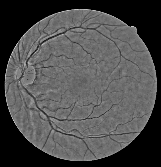
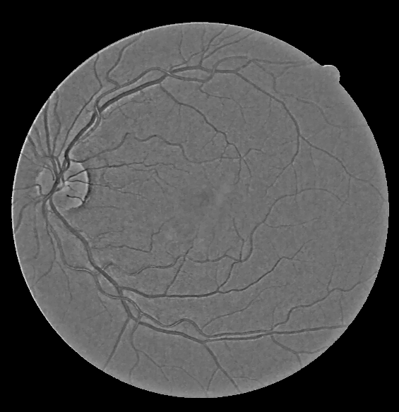
The input image is a combination of noise and structure layers. \begin{equation} I^c(x,y) = I^c_{noise}(x,y) + I^c_{structure}(x,y), c \in (R,G,B) \end{equation}

Noise corresponds to high frequency. TV decomposition method employs a cost function minimization to remove the high frequency layer:

\begin{equation} I^c_{structure}(x,y) = arg min_I \sum_{x,y}^{}\left [ (I(x,y)-I^c(x,y))^2 + \lambda^c\Delta I(x,y) \right ] \end{equation}

In the above equation there are two terms. The first term is called the variation term: which is simply the squared difference between $I(x,y)$ and the input image. The 2nd term is called the regularisation term, which corresponds to the gradient of I. The physical significance is that, to minimize both terms, the output needs to be as close to the input as possible but should not have high frequency edges. Regularisation term $\lambda_c$ corresponds to the degree of smoothness required for the operation, over every color layer in R, G, B.

So for the first step, equations 1 and 2 are followed. $\lambda_c$ is calculated for each color layer $I_c$ from the following equation:

\begin{equation} \lambda^c = \sqrt{\pi/2}\frac{1}{6(W-2)(H-2)}\sum_{x,y}^{}\left | (I^c\star N_s)(x,y) \right | \end{equation}

\begin{equation} N_s = \begin{bmatrix} 1 & -2 & 1\\ -2 & 4 &-2\\ 1 &-2 & 1\\ \end{bmatrix} \end{equation}

W and H correspond to width and height of the image and c refers to each color layer R,G,B. Figure 1 shows the results of input image decomposition into structure layer and noise layer. Scikit-Image provides an inbult function to implement TV decomposition and the same has been used in this process.

2nd decomposition

Moving on to the 2nd step of decomposition, the same method is used. But this time, the practical value of $\lambda $ is kept constant for all layers at 0.3.

\begin{equation} I^c_{structure}(x,y) = I^c_{base}(x,y) + I^c_{details}(x,y), c \in (R,G,B) \end{equation}

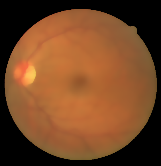
Base lumination correction

For illuminant correction, first the RGB space is converted to HSV space and V layer is extracted as luminance information, denoted as $L_{in}(x,y)$. Correction is done by the following equation, where n is the contrast enhancement parameter. It is set to 1 for all experiments given. \begin{equation} L_{out} = \frac{L_{in}^n}{L_{in}^n+\sigma_g^n} \end{equation} Visual adaptation level is determined by $\sigma_g$,which is a global adaptation level estimated from the whole luminance image from the equation below: \begin{equation} \sigma_g = \frac{M_g}{1+exp(S_g)} \end{equation} where $M_g$ and $S_g$ are the mean and standard deviation of the entire $L_{in}$ respectively. Finally, corrected base is found out by transferring the HSV space back to RGB space.

Detail Layer Enhancement

Red and Green detail layers are passed through a Gaussian filter, keeping in mind that a Gaussian filter is essentially a low pass filter and it will somewhat blur the edges of the veins, making them thicker and more prominent, while removing other noise and artefacts. The execution of the next step differs a bit from the original reference paper. Blue layer does not carry much information and hence is not used.

The enhanced detail layers are merged with the corresponding base layers to form the final output according to the equation: \begin{equation} I_{out}^c = I_{correct-base}^c + \alpha^c I_{enhance-details}^c \end{equation}

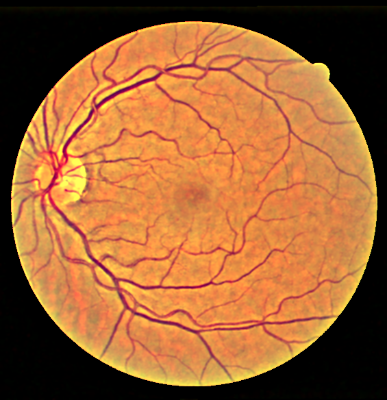
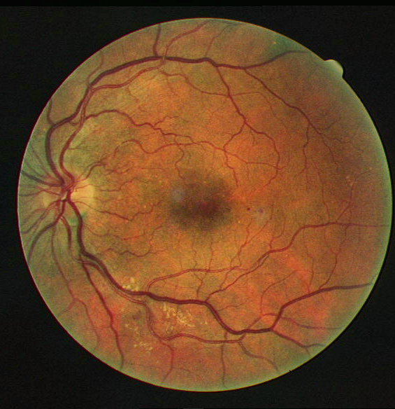
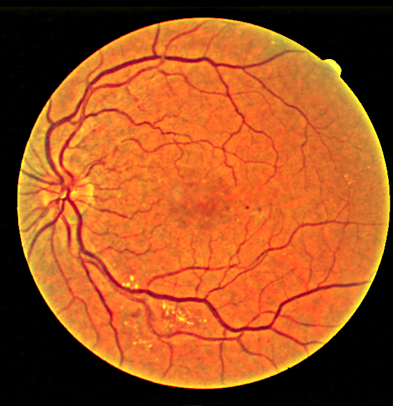
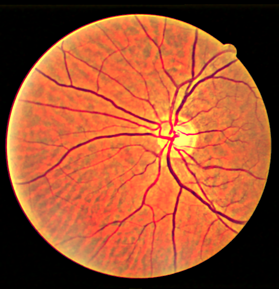
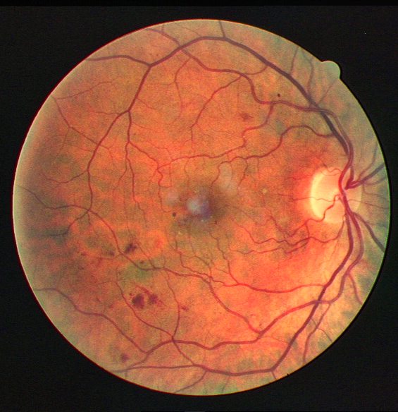
The output is clearly much better than CLAHE visually.

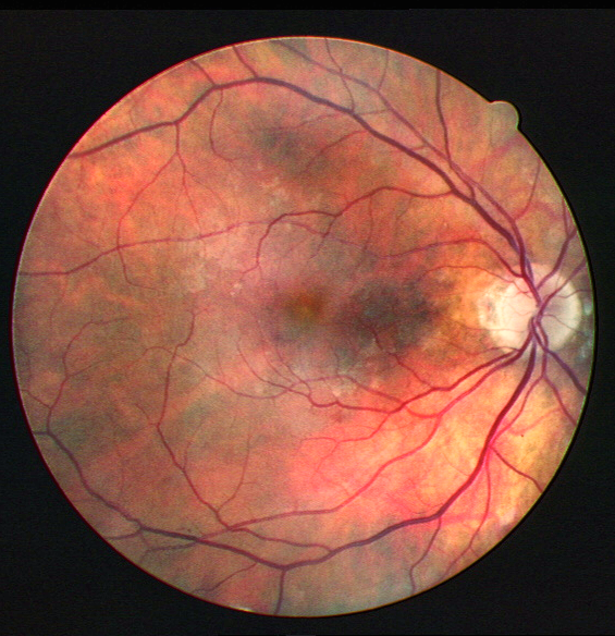
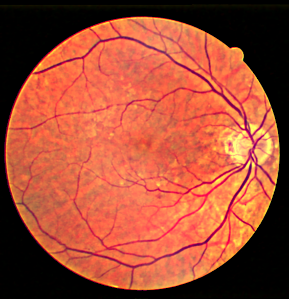
Some more examples for different images, and outputs compared against CLAHE

The code for the project will be uploaded on Github very soon!