Enemies of feature visualisation: High frequency distortions
First understand how feature visualisation works:
Essentialy we choose a random image and iteratively optimise it so that a specific neuron is fired.
STEPS:
- Choose a neuron whose activation you want to visualise.
- Initialise a random image
- Forward propagate: Get the output of the random image at that neuron: We want to maximise this: Our cost function
- Back-propagate on it using Gradient Ascent: Find the gradient with respect to input, add this to the input
Note: in gradient descent> we subtract the gradient from weights during backpropagation.
Ideally this should give the optimised image for that particular neuron: But
High frequency artifacts creep in.
HOW?
Note almost all neurons in a layer are trying to find artifacts/ features from the previous layer output. In gradient ascent we are essentially adding all these features into the image, a bit mindlessly!
So we end up with a kind of neural network optical illusion: image full of noise and nonsensical high-frequency patterns that the network responds strongly to.
In this assignment, we try to remove high frequency artifacts and noise in each iteration using a denoising algorithm:
- Total variation
Total variation denosing method: In TV method we follow an optimization method to minimize the following cost function: $$ min_u \sum_{i=0}^{N-1}((f_i-u_i)^2 + \lambda \left |\Delta u_i \right |) $$ where f is the input image and u is the output(denoised).
The first term is called variation term and 2nd term is regularization.
Look closely: 1st term is difference of input and output image. This can be minimised by just taking input image equal to output image.
But regularisation is provided by the 2nd term: we also have to minimise the gradients of the output image.
On a smallar scale we can think of noise pixels as having high gradient compared to its neighbours. If we smooth out that pixel, we are reducing the gradient.
OVERALL: we want our output to be close to input image, but without high frequency gradients: keep structure of original image and reject the excessive gradients: effectively denoising.
Code in Google Colab
Copy and Run
import numpy as np
import tensorflow as tf
from tensorflow import keras
import matplotlib.pyplot as plt
from IPython.display import Image, display
from tqdm import tqdm
import cv2
from skimage.restoration import denoise_tv_chambolle
model = keras.applications.ResNet50V2(weights="imagenet", include_top=True)
layer_name = "conv5_block1_out"
img_width, img_height = 224, 224
# Set up a model that returns the activation values for our target layer
layer = model.get_layer(name=layer_name)
feature_extractor = keras.Model(inputs=model.inputs, outputs=layer.output)
Initialise the random image
def initialize_image():
    # We start from a gray image with some random noise
    img = tf.random.uniform((1, img_width, img_height, 3))
    # ResNet50V2 expects inputs in the range [-1, +1].
    # Here we scale our random inputs to [-0.125, +0.125]
    return (img - 0.5) * 0.25
Loss function is effectively the mean of activation at a particular neuron
Maximize this loss
def compute_loss(input_image, filter_index):
    activation = feature_extractor(input_image)
    # We avoid border artifacts by only involving non-border pixels in the loss.
    filter_activation = activation[:, 2:-2, 2:-2, filter_index]
    return tf.reduce_mean(filter_activation)
@tf.function
def gradient_ascent_step(img, filter_index, learning_rate):
    with tf.GradientTape() as tape:
        tape.watch(img)
        loss = compute_loss(img, filter_index)
    # Compute gradients.
    grads = tape.gradient(loss, img)
    # Normalize gradients.
    grads = tf.math.l2_normalize(grads)
    img += learning_rate * grads
    return loss, img
def deprocess_image(img):
    # Normalize array: center on 0., ensure variance is 0.15
    img -= img.mean()
    img /= img.std() + 1e-5
    img *= 0.15

    # Center crop
    img = img[25:-25, 25:-25, :]

    # Clip to [0, 1]
    img += 0.5
    img = np.clip(img, 0, 1)

    # Convert to RGB array
    #img *= 255
    #img = np.clip(img, 0, 255).astype("uint8")
    return img

def visualize_filter(filter_index, learning_rate, iterations, blur, blur_weight):
    num = [5,10,50,100,200,500,750, 1000, 1500, 2000]
    image_array = []
    img = initialize_image()
    for iteration in tqdm(range(iterations)):
        loss, img = gradient_ascent_step(img, filter_index, learning_rate)
        #print(img.shape)
        if (blur == True):
            if (iteration>=50):# and iterations<1000):
                #print('yes hello')
                img = img.numpy()
                img = denoise_tv_chambolle(img, weight = blur_weight)
                img = tf.convert_to_tensor(img)

        if (iteration in num):
           # print(iteration)
            image_array.append(deprocess_image(img[0].numpy()))


    return loss, image_array
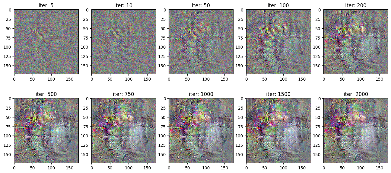
num_array = [5,10,50,100,200,500,750, 1000, 1500, 2000]
loss, image_array0 = visualize_filter(1, learning_rate = 2.0, iterations = 2001, blur = False, blur_weight = 0)
plt.figure(figsize = (16,7))
for i in range(10):
    plt.subplot(2,5,i+1)
    plt.imshow(image_array0[i])
    plt.title('iter: '+str(num_array[i]))
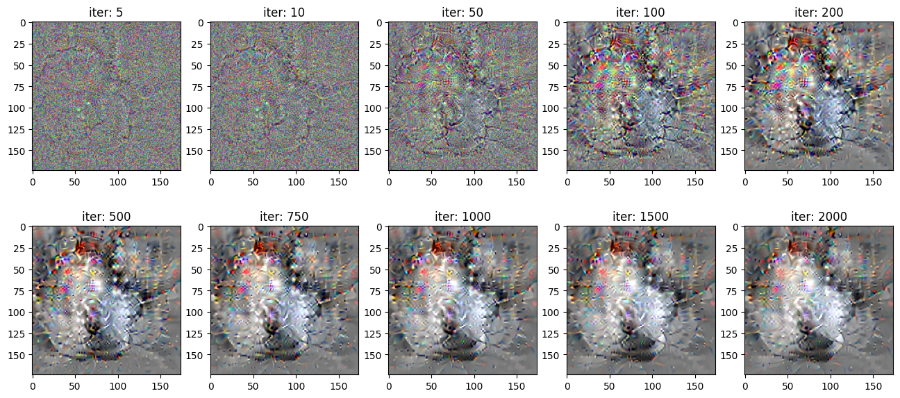
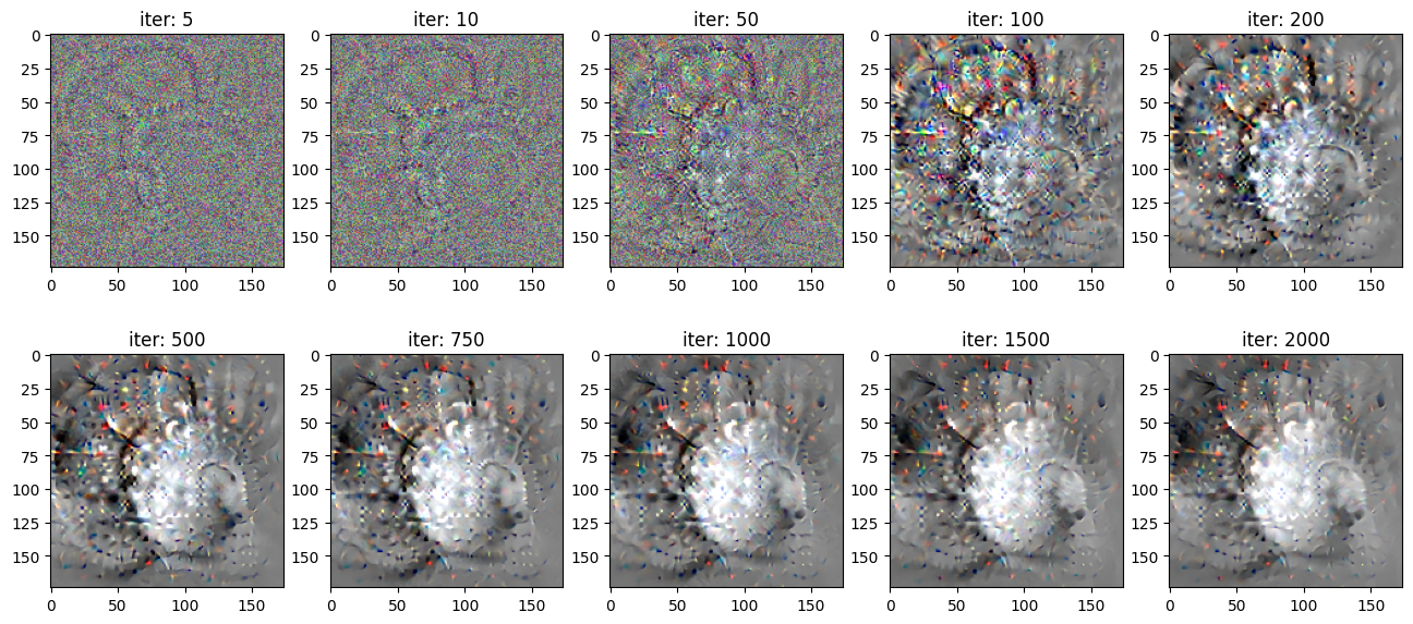
loss, image_array01 = visualize_filter(1, learning_rate = 2.0, iterations = 2001, blur = True, blur_weight = 0.0005)
num_array = [5,10,50,100,200,500,750, 1000, 1500, 2000]
plt.figure(figsize = (16,7))
for i in range(10):
    plt.subplot(2,5,i+1)
    plt.imshow(image_array01[i])
    plt.title('iter: '+str(num_array[i]))
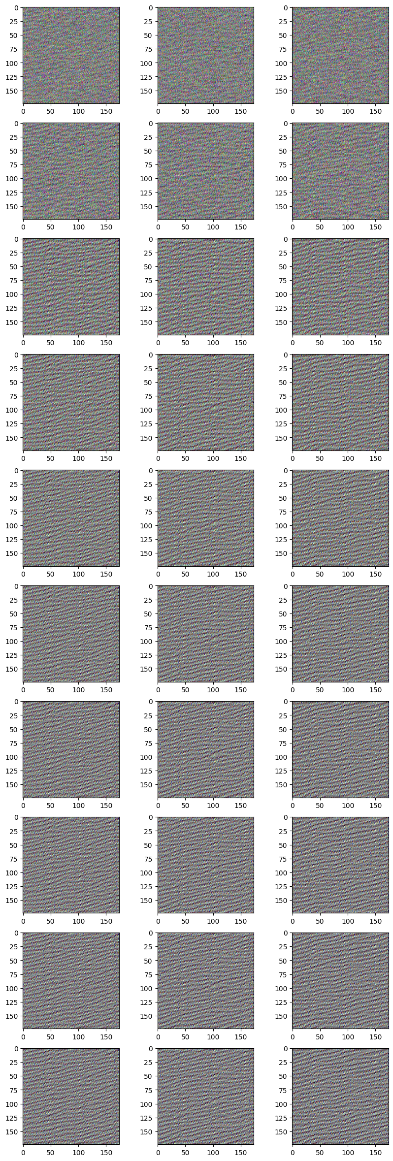
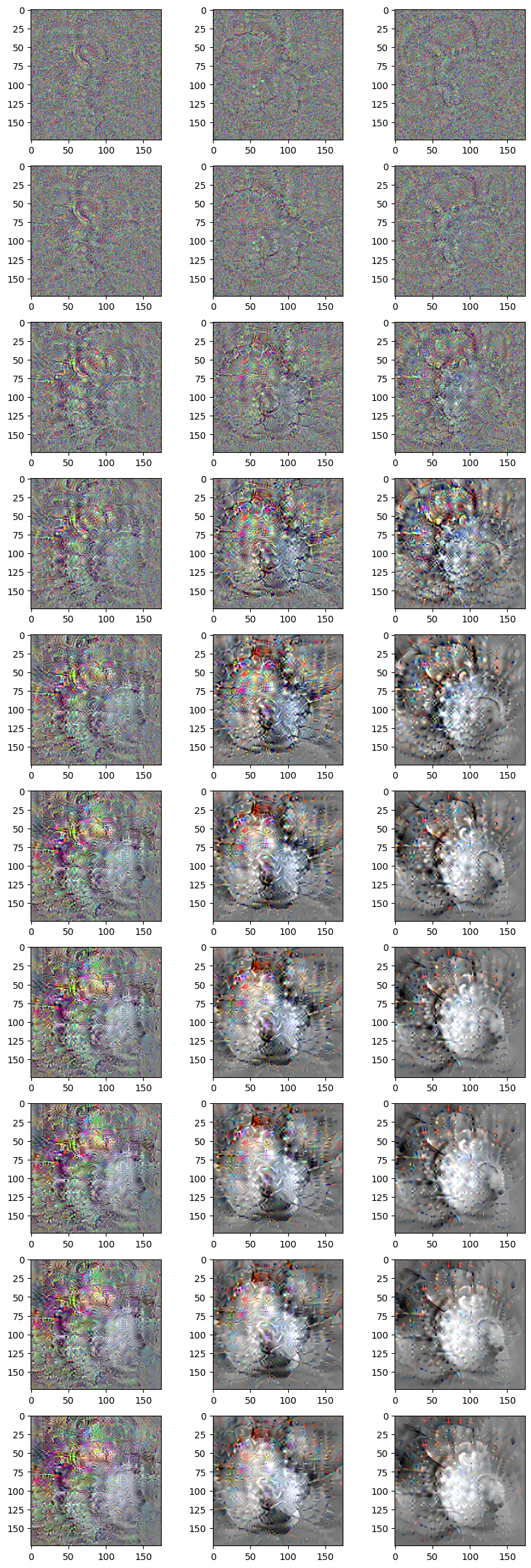
Compare between different denoise parameters
Block 5 Conv 3
This neuron detects a superposition of circles/curves.
1st column: no denoising
2nd column: denoising parameter 0.0005
3rd column: denoising parameter 0.001
Block 2 Conv 2
This particular nueron detects diagonal/curvy lines.
Towards the initial layers, not much noise is added and thus there is not much effect of denoising.